
Have you heard about quantum numbers or states? How about eigenvalues? How about wave functions? How about Schrodinger’s equation (no, not the cat, the actual equation)? Or how about Heisenberg’s Uncertainty Principle? No? Doesn’t ring a bell? That means you have been spared from taking Quantum Mechanics in university. Not to worry. You can grasp what you need to know about Quantum Computing if you know a bit of math and are open to lateral thinking.
Basic concepts
The basic new concepts you need:
- The Qubit: like a bit, but with the extra perk that it can be 0, 1 or a bit of BOTH (see Superposition below). The value 0 and 1 are typically two different quantum states of a particle. A common example is the spin-up or spin-down in an electron.
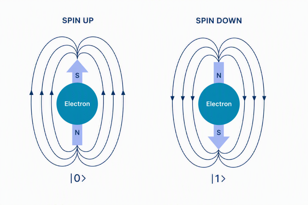
In quantum physics, we represent these two quantum states as follows:
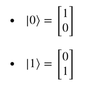
We call |0> and |1>, ket 0 and ket 1 respectively (Dirac notation).
An electron’s spin can be oriented in any direction in the physical world. To fully describe its position, we require a 3D diagram. You may sometimes find Bloch Sphere representations to depict the quantum state of an electron’s spin (|ψ⟩). On the z-axis, we have the reference direction for spin up |0> (north) and down |1> (south). The actual spin position can be described with two values θ (amplitude) and ϕ (phase). The point represented by θ and ϕ is unique.
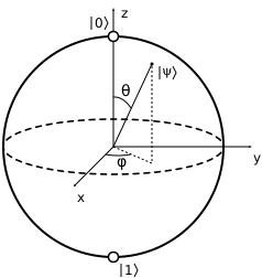
The actual quantum state of the spin of an electron is not known until we measure it. Until then we can only talk about superposition of states.
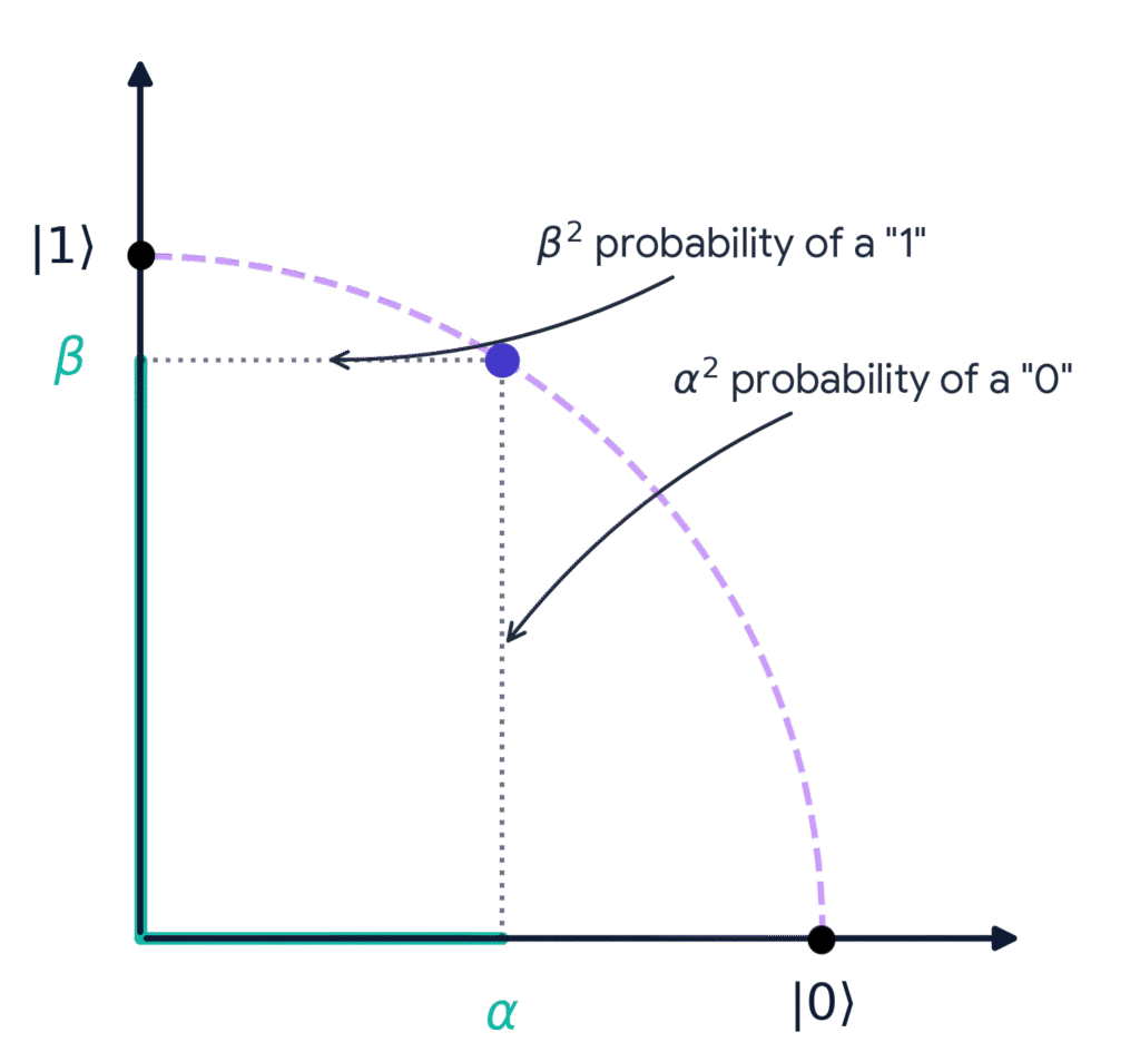
- Superposition: In the quantum world, we work with probabilities of quantum states, not absolutes. We can ask: is the traffic light red or green? In quantum mechanics, the answer is BOTH until we look (and realise we just went through a yellow/orange and may get a ticket). Only when we measure (look at the traffic light) does the wave function collapse into a given value. Until then, we have a superposition of quantum states. Before we measure its state, the qubit is both in state |0> and state |1>, and we can only calculate the probability that it will collapse into one or the other. When we measure (look) at the state of the qubit, its quantum state will collapse into |0> or |1> at the probability rate we calculated.
We represent this superposition as follows:
|𝜓> = 𝛼|0>+𝛽|1>: superposition of states |0> and |1>
𝛼2 = probability that the wave function will collapse into a |0> state
𝛽2 = probability that the wave function will collapse into a |1> state
The famous thought experiment with the cat (Schrodinger’s cat) is a way of showcasing how the quantum superposition phenomenon is not applicable to anything other than basic particles.
- Entanglement: Ah… this happens to me sometimes when I crochet 🙂. But it can also happen at a quantum level. And it gets spooky (a term used by Einstein to describe this phenomenon). Entanglement means that two particles (or more) can become “linked” (or quantum entangled). Their states have a certain connection. And if you separate them, that connection remains. Entangled particles are considered to be part of a single system. Properties of such particles are correlated since the moment of their entanglement, and that correlation is not lost over time or space. A common example used is that if you have two electrons entangled such that they have opposite spin, when you measure one and it turns out to be in state |0>, you know, without measuring, that the other one is in state |1>. No matter how much time and distance has been put between them, that relation of having opposite spins remains.
The first two concepts – qubit and superposition – are central to the operation of a quantum computer. Entanglement plays a role in communications. With this new concept of qubits, we have a way of “jotting down” some data, and superposition enables us to process several variables at once. But how do we execute mathematical operations on those values? Enter the quantum gates.
Quantum gates
If you are familiar with the concept of logical gates (AND, OR, XOR, NOT,…), then quantum gates represent the same concept but for qubits.
These are a few of the quantum gates used in quantum computing:
- Pauli X gate: your basic NOT operation. It will rotate a spin-up to spin-down and vice versa. But because we are now operating in a 3D environment, we have a couple of ways of executing this action. This is a rotation around the x-axis.
- Pauli Y gate: also a NOT operation. It will rotate a spin-up to spin-down and vice versa. This is a rotation around the y-axis.
- Pauli Z gate: a rotation around the z-axis. This is called changing the phase of the particle. However, it does not flip the quantum state.
- Hadamard gate: changes a qubit to a neutral state with a 50/50 chance it will collapse into a |0> or |1> state.
- T gate: rotates a qubit by 𝜋/4 around the z-axis.
- Controlled NOT gate: utilises a control qubit. If the control qubit is set to |1>, it will operate as a NOT gate. If the control qubit is |0>, it does nothing. As an extra note, the CNOT gate will result on the control and input qubits being entangled.
- SWAP gate: The swap gate swaps two qubits
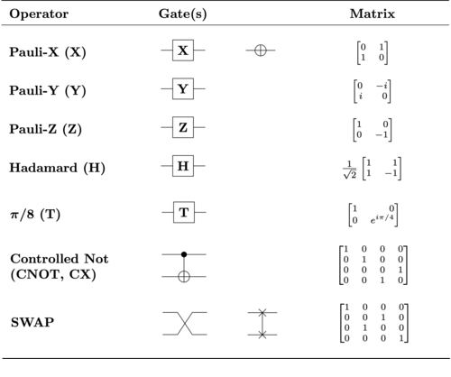
There are more gates examples which can execute more complex operations. Quantum gates are reversible and operate on a single qubit.
In reality, these gate computations are done by applying precise energy pulses on the target qubit (using microwave, lasers, magnetic fields). The target qubit will change its quantum state based on this external influence and so will the probability of it being in a |0> or |1> state when measured.
Qubits and quantum gates together give us quantum computing.
If you want to try creating algorithms using qubits and quantum gates, read the blog posted on the Conscia website. There you will find some tips on how to get started on a simulated environment or even “borrow” a real quantum computer.
In the next blog, I will cover the performance of quantum computing systems as well as why they are relevant in the cryptography field.